Electromagnetic Induction

Step 1: Understanding the Magnetic Field and Torque

We are dealing with a small circular loop of area and resistance , placed in a solenoid carrying a time-varying current. The magnetic field inside the solenoid is given by , where is the amplitude of the magnetic field, and is the angular frequency.

The torque on the loop is given by: where is the magnetic moment of the loop, and is the magnetic field. The time-varying magnetic field induces a torque on the loop, which varies with time.

Step 2: Analyzing Column I Expressions

The expressions in Column I represent the time-varying magnetic field and the corresponding torques in Column II.

Expression I:
This expression represents the time-varying magnetic field. Since both the sine and cosine terms oscillate with the same frequency, their combination results in a net zero average torque over one complete cycle. Therefore, the torque corresponding to this field is , which indicates zero torque.

Expression II:
This expression is similar to Expression I. Given the same sinusoidal time-dependence, the net torque is again zero over one complete cycle, so the corresponding torque is , which is also zero.

Expression III:
This time-varying field produces a torque that is proportional to the angular frequency , which gives a non-zero torque that oscillates. The corresponding torque expression is .

Expression IV:
Like Expression III, this expression also results in a non-zero torque but with a different time-dependence. The corresponding torque expression for this is .

Step 3: Final Answer

Based on the analysis, the correct matching is:

• Expression I corresponds to torque (zero torque),
• Expression II corresponds to torque (zero torque),
• Expression III corresponds to torque ,
• Expression IV corresponds to torque .

Final Answer: The correct option is: C: I → Q, II → P, III → S, IV → R.

Background Physics:

• Faraday's Law: As the loop enters the magnetic field, there's a changing magnetic flux, inducing an emf (electromotive force) in the loop.
• Ohm's Law: The induced emf drives a current through the loop.
• Lenz's Law: The induced current creates a magnetic force that opposes the motion of the loop entering the field. This is the retarding force.
• Force on a current-carrying wire: , where is the length of the wire in the field.
• Newton's Second Law: The net force on the loop affects its acceleration and velocity.

Derivation of Equation of Motion

Let be the distance the loop has entered the magnetic field at time .

1. Induced EMF: , where .
2. Induced Current: .
3. Magnetic Force: (with ).
4. Equation of Motion: .
5. Solving for : .
6. Solving for : .

Statement A: If , the loop will stop before entering completely into the field.

We know that as , . For , we get , so the loop does enter fully. A is incorrect.

Statement B: When the entire loop is inside the magnetic field, the induced emf becomes zero since there's no change in flux. Hence, current and magnetic force also become zero. B is correct.

Statement C: Analyzing the given at :

This is far less than , so the loop has barely entered. C is incorrect.

Statement D: To find when , set:

Thus, D is correct.

To solve this problem, we need to determine the induced electromotive force (e.m.f., ) in a square loop rotating in a time-varying magnetic field. Let’s break it down step by step.
Step 1: Understand the Setup

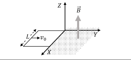
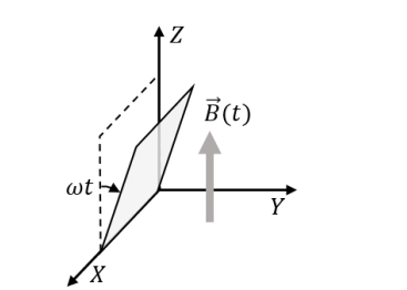
• The square loop lies in the -plane at , with its lower edge hinged along the -axis.
• The loop rotates with a constant angular speed about the -axis in the clockwise direction (as viewed from the positive -axis). Clockwise rotation from this perspective means the loop rotates from the -axis toward the negative -axis.
• The magnetic field exists only in the region and is given by , where is a constant, and is the unit vector along the -axis. The field is zero for .
• We need to find the induced e.m.f. as a function of time and match it with the given plots.

Step 2: Define the Loop’s Position and Area Vector Assume the square loop has a side length , so its area is . At , the loop lies in the -plane, meaning its area vector (normal to the plane) points along the -axis (positive -direction, ). The loop rotates about the -axis with angular speed . The angle of rotation at time is: Since the rotation is clockwise as viewed from the positive -axis, the loop’s plane tilts from the -plane (where the normal is along ) toward the negative -axis. Let’s define the position:

• At , the loop is in the -plane, and the area vector .
• After time , the loop has rotated by an angle . The normal vector (area vector direction) rotates in the -plane.

The normal vector’s direction after rotation: Initially (at ), the normal is along . After rotating by clockwise (from to ), we can determine the new normal using the rotation matrix about the -axis. For a clockwise rotation by about the -axis: The initial normal is .

After rotation:
So, the area vector becomes:

Step 3: Calculate the Magnetic Flux The magnetic flux through the loop is: The magnetic field is , and it exists only in the region . This complicates things because part of the loop may be in , where . Let’s first compute the flux assuming the field were uniform across the loop, then adjust for the condition: So, if the field were uniform: However, the field is only present for . As the loop rotates, its position in the -coordinate changes:

• At , the loop is in the -plane ( ), so the entire loop is at the boundary of the field region.
• As increases, the loop tilts, and the -coordinate of points on the loop ranges from 0 (at the hinged edge along the -axis) to at the opposite edge (since it moves toward the negative -axis).

When , the loop is entirely at , so it’s in the field region. When , the loop is in the -plane, with ranging from 0 to , so half the loop (on average) is in , where .

Step 4: Adjust for the Field Region The flux depends on the area of the loop in the region . Let’s parameterize the loop:

• The loop’s hinged edge is along the -axis (from to , , ).
• The opposite edge, initially at , rotates. Its -coordinate becomes , and .

As the loop rotates, the -coordinate of a point at height (before rotation) becomes: The original -coordinate ranges from 0 to . So, ranges from 0 to . The condition means: Since , when , no part of the loop satisfies except at the hinge ( ). This suggests we need to compute the effective area in . Instead, let’s reconsider the flux by integrating over the loop’s surface. The fraction of the loop in decreases as increases. At , ranges from 0 to , so half the loop is in . The effective area in the field region depends on the angle.
Step 5: Induced e.m.f. The induced e.m.f. is given by Faraday’s Law: Let’s approximate the flux by considering the effective area. Notice the field and rotation have the same frequency , suggesting resonance effects. Let’s compute using the uniform flux and adjust: This e.m.f. oscillates with frequency , which matches the period in the plots ( ).
Step 6: Account for Condition When , the loop is half in , so the flux is halved, but the derivative (e.m.f.) depends on the rate of change. The form arises from the product of (from the field) and (from the area vector’s -component), and the condition modulates the amplitude, not the frequency.
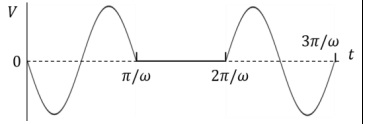
Step 7: Match with Plots

• The e.m.f. has a period of .
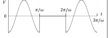
• Option (A) shows a period of , matching .
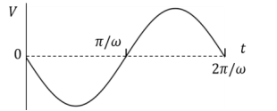
• Option (B) shows a period of , incorrect.
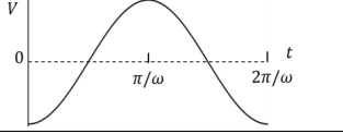
• Option (C) shows a period of , incorrect.
• Option (D) shows a period of , but the phase differs.

Since starts at a maximum, option (A) matches best.
Final Answer